K-maps
Table of contents
- Introduction
- Enumeration and gray codes
- Simple groupings
- Two dimension groupings
- Disjoint groupings
- Overlapping groupings
- Minimizing group count
Introduction
Karnaugh Maps are a way to visually display a boolean expression onto a 2D grid. Take the variables and bind them to an axis, and then enumerate through the possible combinations of input values that could occur for all those variables bounded to an axis (either horizontally or vertically).
For example, display the following 2 variable Karnaugh Map:
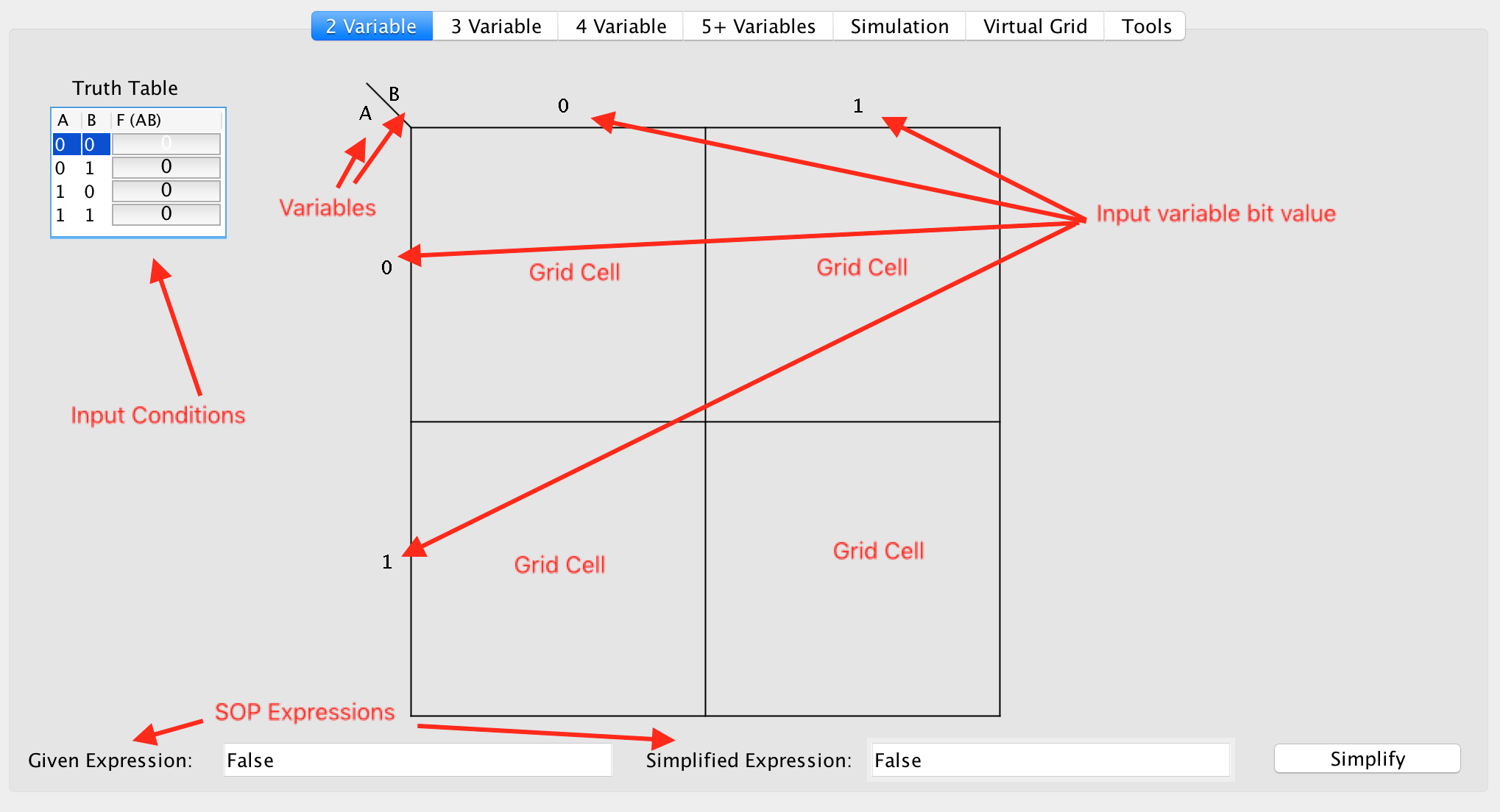
You have bounded to the vertical axis, the variable A, and enumerate through the possible values for A (being {0, 1}). Similarly, perform a similar operation for the B variable. Since you are using a 2 variable expression, you can bound one variable to each axis and the visualization works fine in a 2x2 matrix.
Let’s instead look at a more involved example with 4 variables:
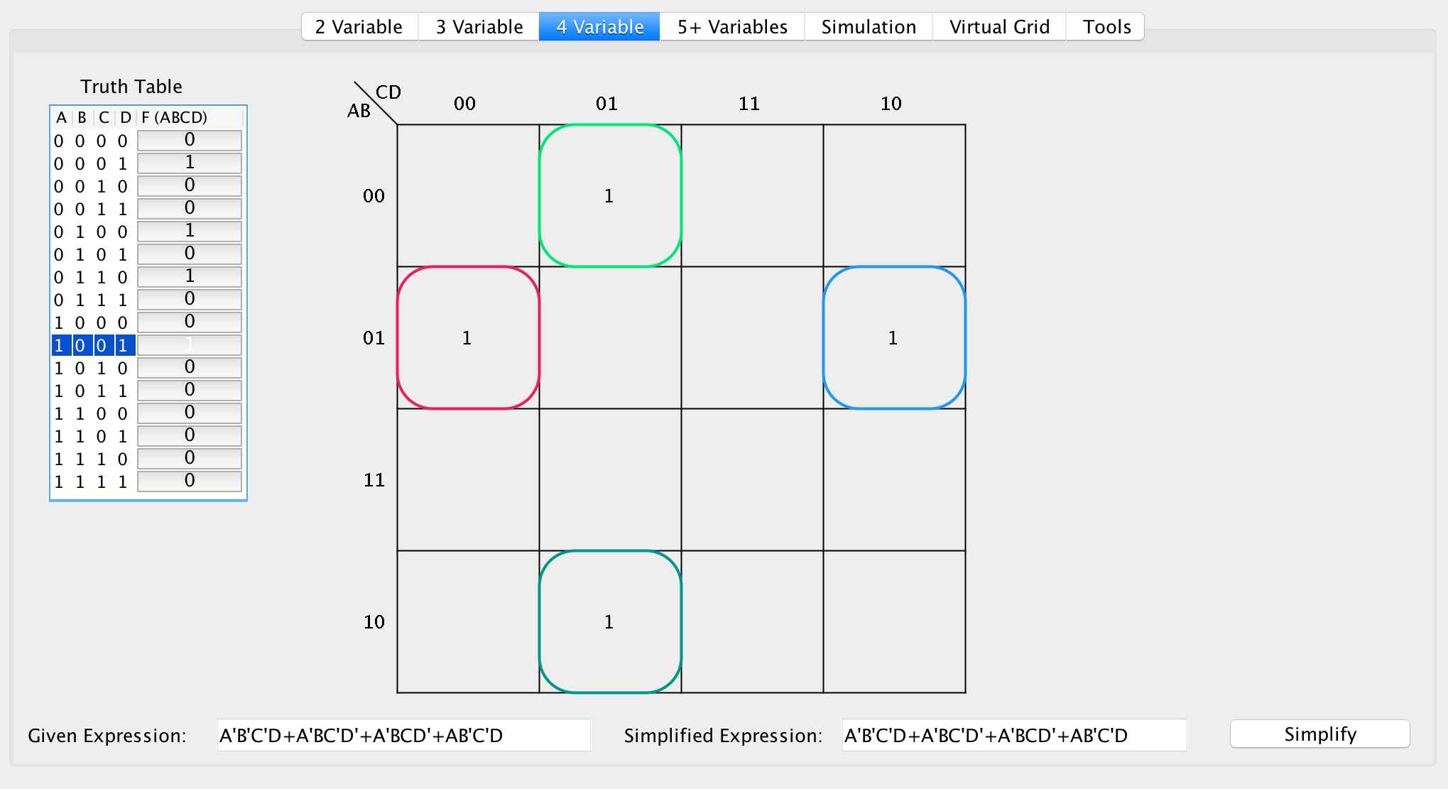
You have now bounded the A and B variables to the vertical axis, and C and D variables to the horizontal axis. Now enumerate through different combinations of the bounded variables for each axis in reflected binary code order (more on this in the following section). Lastly, indicate on the matrix each true value by augmenting a 1 value.
Enumeration and gray codes
When enumerating through the variable input combinations for the bound axis, we take advantage of reflected binary code order, otherwise known as grey codes. If we observe, we can notice that from one combination to another, we only vary by one bit. That is:
... 00 01 11 10 00 01 11 10 00 ...
    ^   ^ ^   ^ ^   ^ ^   ^ ^
Thus, you get this wrapping that allows us to switch by only one bit. This provides us with the core of how Karnaugh Maps work.
Simple groupings
The main idea for how Karnaugh Maps can be used to simplify expressions is to group pairs of 1 values that are adjacent and exploit the fact that each one has only a bit different from another.
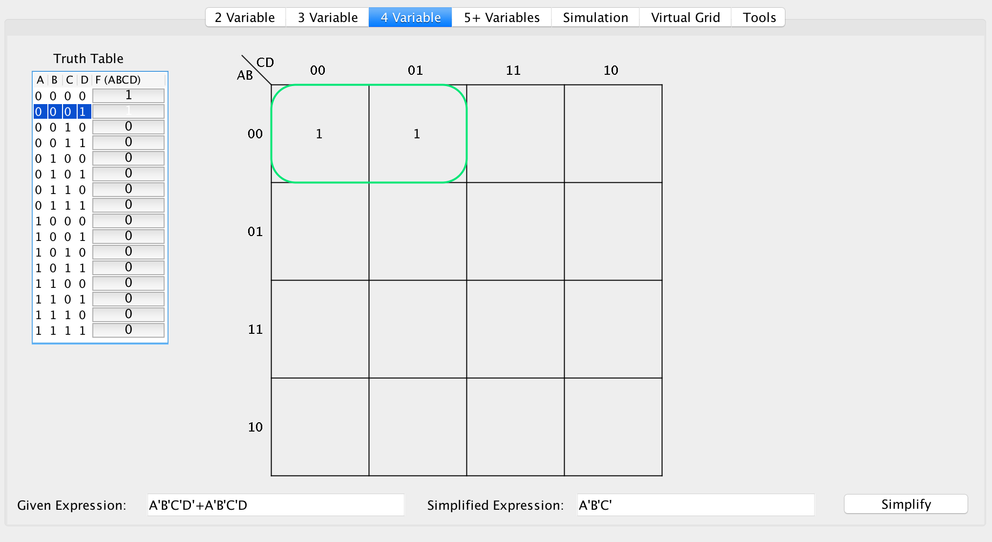
For this example, let F(ABCD) = CELL. start with the expression F(0000) = 1 and F(0001) = 1. However, notice that regardless of the value of the last bit, you still get 1. Hence, let’s take a look at the SOP expressions:
F(ABCD) = A'B'C'D' + A'B'C'D
F(0000) = 1
F(0001) = 1

Since the last bit is the same, you can ignore the D value, thus:
F(ABCD) = A'B'C'

You can confirm by simplifying algebraically:
F(ABCD) = A'B'C'D' + A'B'C'D
      = A'B'C'(D' + D)
      = A'B'C'
Therefore, the simplification is true.
You can then extend this rule to work for rectangles and more!
Two dimension groupings
Extending the idea of isolating changing bits that retain a consistent value, we can then generalize this to work in a higher dimension. Consider the following example:
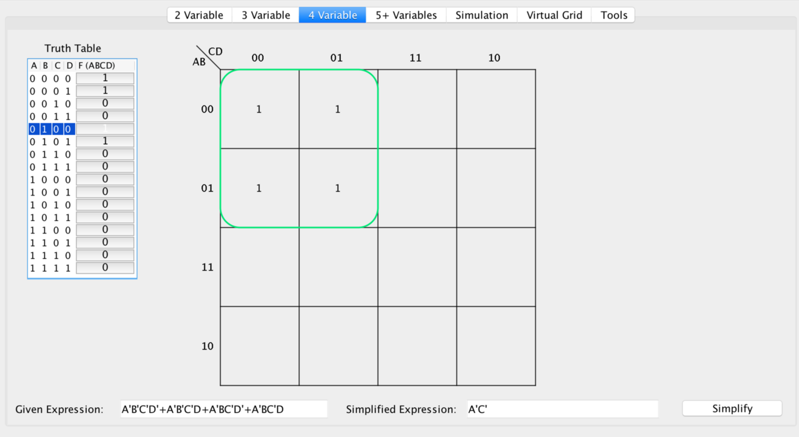
Letting F(ABCD) = CELL:
F(0000) = 1
F(0001) = 1
F(0100) = 1
F(0101) = 1
Observe that the bits do not change by one for all pairs of numbers, for example, {0000, 0101} differ by two bits. However, you can take advantage of the fact that for any bit change horizontally or vertically, it’s irrelevant what that bit is. More concretely, take a look at the following example.
0000 0001
0100 0101

=> A'B'C'D' + A'B'C'D + A'BC'D' + A'BC'D
Regardless of the B variable, you still get true for all products in the SOP expression.
This is bounded vertically:
=> A'C'D' + A'C'D + A'C'D' + A'C'D
Regardless of the D variable, you still get true for all products in the SOP expression.
This is bounded horizontally:
=> A'C' + A'C' + A'C' + A'C'
=> A'C' (1 + 1 + 1 + 1)
=> A'C' (1)
=> A'C'
Since the differences in bits need to generalize throughout a binding of an axis, you can only have a binding of size 2^n for a given axis. For example, 1x1, 1x2, 1x4, 2x2, 2x4, 4x4.
Disjoint groupings
Consider the following example: 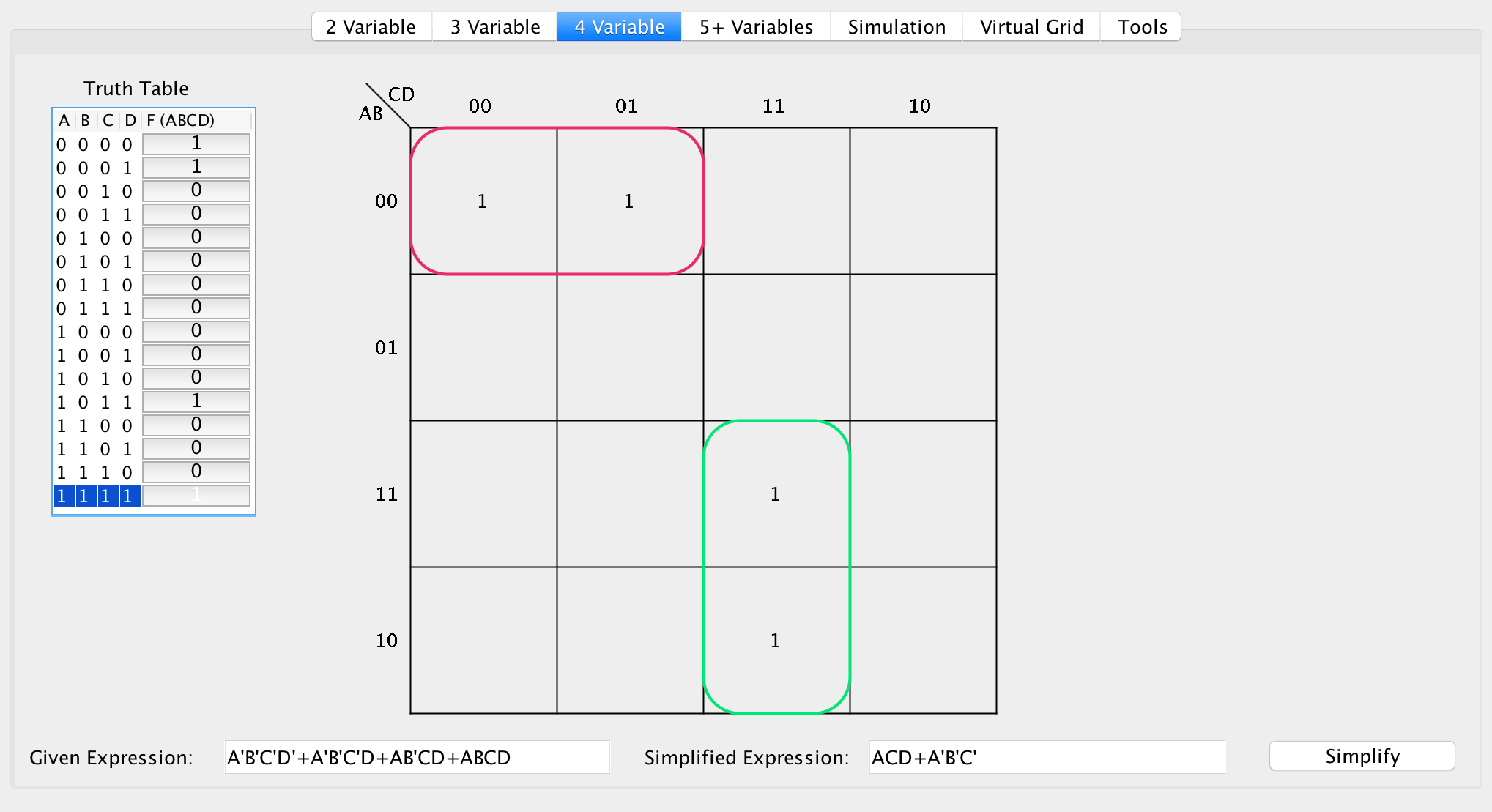
The algorithm follows precisely as it did before, except that now the two groups are joined in the SOP expression. Letting F(ABCD) = CELL:
F(0000) = 1
F(0001) = 1
F(1111) = 1
F(1011) = 1
This yields the following:
A'B'C'D' + A'B'C'D + ABCD + AB'CD
Breaking down the expression:
(A'B'C'D' + A'B'C'D) + (ABCD + AB'CD)
=> (A'B'C'(D + D')) + (ACD(B + B'))
=> (A'B'C') + (ACD)
=> A'B'C' + ACD
Clearly this is the exact same process as before, but iterated throughout all the disjoint sets.
Overlapping groupings
Overlapping groupings become more complex because there exist ambiguous cases and sometimes what may appear to be a locally optimal solution is not a globally optimal solution.
The general technique for evaluating for overlapping groups follows a greedy algorithm. Define an unvisited cell as a cell that has a value of 1 however it is currently not matched with a grouping yet.
Iterate through all the cells, and once you find a cell with 1, if it is unvisited then find the largest possible square or rectangle such that each side length is a power of 2, where all the cells are 1 in its enclosed area. If there is a tie for size (ie, 1x4 vs 2x2), assign the one that is a square (this is by convention).
Repeat this process for all remaining unvisited cells.
Note: You can overlap the groupings with already visited nodes, but you never instantiate a new grouping unless the current node is unvisited.
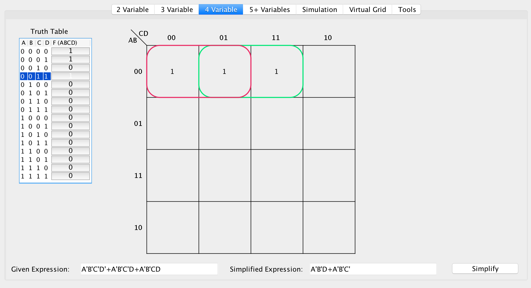
In this example, at F(0000), you can create a grouping of size 2 (because 2 is the largest possible grouping, 3 is not a power of 2). Then iterate through to F(0001), however F(0001) was already resolved to a grouping. For the latest active cell, F(0011) is not resolved to a grouping thus it’s unvisited. The largest possible grouping is also of size 2, thus you create another group.
To resolve the groupings into an SOP expression, iterate through the groups and identify changing bits:
Group 1: F(ABCD) = [0000, 0001]
Group 2: F(ABCD) = [0001, 0011]

For Group 1:
0000 0001
   ^    ^
F(ABCD) = A'B'C'D' + A'B'C'D
=> A'B'C'(D + D')
=> A'B'C'

For Group 2:
0001 0011
  ^    ^
F(ABCD) = A'B'C'D + A'B'CD
=> A'B'D(C' + C)
=> A'B'D

Now add the two results:
F(ABCD) = A'B'C' + A'B'D
=> F(ABCD) = A'B'D + A'B'C' (by commutative property)
Minimizing group count
The following example will illustrate how the greedy approach may occasionally produce too many groups. Consider the following example:
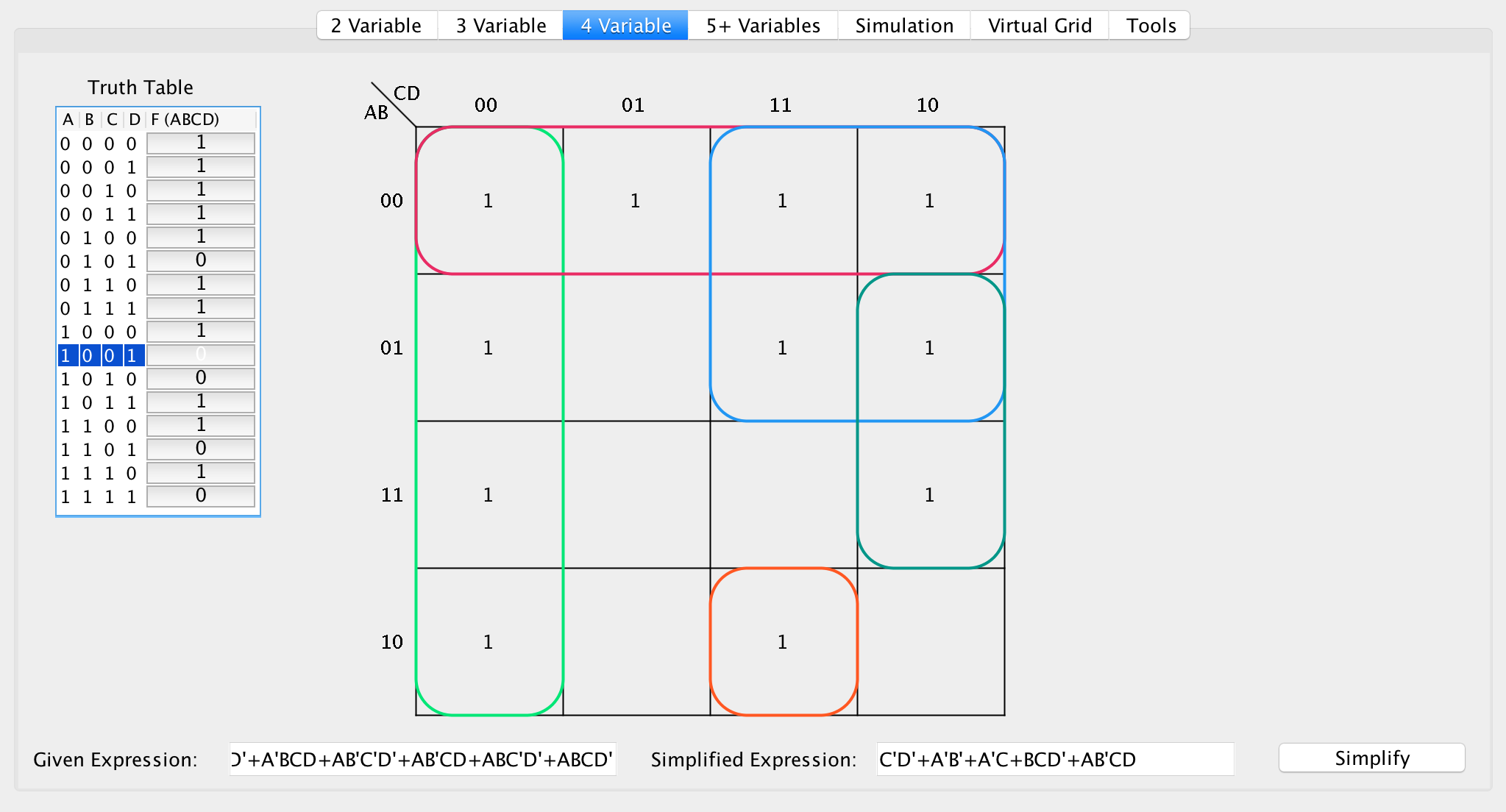
This grouping state is optimal. However, consider adding a 1 to F(1111).
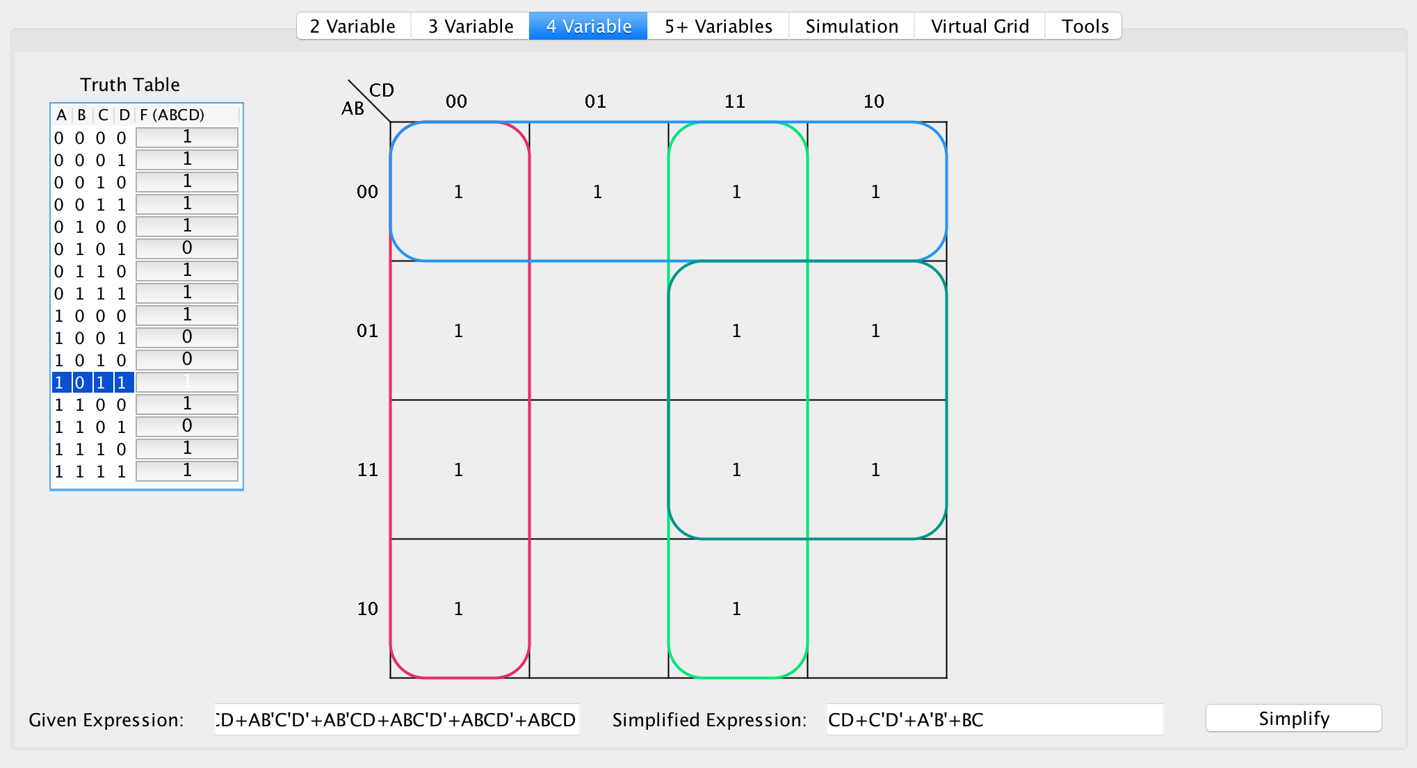
Following the previous algorithm, iterating top-bottom and left-right, when getting to F(0110), the algorithm can choose to make the largest grouping. However, there are two possible groupings:
Candidate 1:
F(ABCD) = [0011, 0010, 0111, 0110]

Candidate 2:
F(ABCD) = [0111, 0110, 1111, 1110]
Both groupings have the same size and are the same dimension. However, upon reaching F(1110), another grouping needs to be instantiated, in which case if the first candidate grouping was created then you made a group that did not necessarily increase the size of our SOP expression.
This illustrates the idea that this is a greedy algorithm, and does not always return the most simplified SOP expression. In later sections, algorithms illustrating a globally optimal algorithm will be discussed.